- Research
- Open access
- Published:
Generating normal networks via leaf insertion and nearest neighbor interchange
BMC Bioinformatics volume 20, Article number: 642 (2019)
Abstract
Background
Galled trees are studied as a recombination model in theoretical population genetics. This class of phylogenetic networks has been generalized to tree-child networks and other network classes by relaxing a structural condition imposed on galled trees. Although these networks are simple, their topological structures have yet to be fully understood.
Results
It is well-known that all phylogenetic trees on n taxa can be generated by the insertion of the n-th taxa to each edge of all the phylogenetic trees on n−1 taxa. We prove that all tree-child (resp. normal) networks with k reticulate nodes on n taxa can be uniquely generated via three operations from all the tree-child (resp. normal) networks with k−1 or k reticulate nodes on n−1 taxa. Applying this result to counting rooted phylogenetic networks, we show that there are exactly \(\frac {(2n)!}{2^{n} (n-1)!}-2^{n-1} n!\) binary phylogenetic networks with one reticulate node on n taxa.
Conclusions
The work makes two contributions to understand normal networks. One is a generalization of an enumeration procedure for phylogenetic trees into one for normal networks. Another is simple formulas for counting normal networks and phylogenetic networks that have only one reticulate node.
Background
Phylogenetic networks have been used to date both vertical and horizontal genetic transfers in evolutionary genomics and population genetics in the past two decades [1–3]. A rooted phylogenetic network (RPN) is a directed acyclic digraph in which all the sink nodes are of indegree 1 and a unique source node is designated as the root, where the former represent a set of taxa (e.g, species, genes, or individuals in a population) and the latter represents the least common ancestor of the taxa. Moreover, the other nodes in a RPN are divided into tree nodes and reticulate nodes, where reticulate nodes represent reticulate evolutionary events such as horizontal genetic transfers and genetic recombination.
The topological properties of RPNs are much more complicated than phylogenetic trees [2, 4, 5]. Therefore, different mathematical issues arise in the study of RPNs. First, phylogenetic reconstruction problems are often NP-hard even for trees [6, 7]. As such, a phylogenetic reconstruction method often uses nearest neighbor interchanges (NNIs) or other rearrangement operations to search for an optimal tree or network [8, 9]. Recently, different variants of NNI have been proposed for RPNs [10–16].
Second, to develop efficient algorithms for NP-complete problems on RPNs, simple classes of RPNs have been introduced, including galled trees [17, 18], tree-child networks (TCNs) [19], normal networks [20], reticulation-visible networks [4] and tree-based networks [21, 22] (see also [5, 23]). For instance, a RPN is a TCN if every non-leaf node has a child that is a tree node or a leaf. Although these network classes have been intensively investigated, their topological structures remain unclear [5, 24]. How to efficiently enumerate and count normal networks remains unclear [25–30].
This work makes two contributions to understanding TCNs and normal networks. It is a well-known fact that all phylogenetic trees on n taxa can be generated by inserting the n-th taxa in every edge of all the phylogenetic trees on n−1 taxa. We prove that all TCNs with k reticulate nodes on n taxa can be uniquely generated via three operations from TCNs with k−1 or k reticu- late nodes on n−1 taxa (Theorem 1, “Generating TCNs and normal networks” section). Using this fact, we obtain recurrence formulas for counting TCNs and normal networks (“Counting formulas” section). In particular, simple formulas are given for the number of RPNs and normal networks with one reticulate node, respectively.
Methods
Basic notation
A RPN over a finite set of taxa X is an acyclic digraph such that:
there is a unique node of indegree 0 and outdegree 1, called the root;
there are exactly |X| nodes of outdegree 0 and indegree 1, called the leaves of the RPN, each being labeled with a unique taxon in X;
each non-leaf/non-root node is either a reticulate node that is of indegree 2 and outdegree 1, or a tree node that is of indegree 1 and outdegree 2; and
there are no parallel edges between a pair of nodes.
Two RPNs are drawn in Fig. 1, where each edge is directed away from the root and both the root and edge orientation are omitted. For a RPN N, we use \({\mathcal {V}}(N), {\mathcal {R}}(N), {\mathcal {T}}(N)\) and \({\mathcal {E}}(N)\) to denote the set of all nodes, the set of reticulate nodes and the set of tree nodes and the set of directed edges for N, respectively.

Two tree-child networks on {1,2,3,4,5}, where reticulate and tree nodes are drawn as filled and unfilled circles, respectively. Only the right network is normal. Here, edge downward orientation is omitted
Let \(u\in {\mathcal {V}}(N)\) and \(v\in {\mathcal {V}}(N)\). The node u is said to be a parent (resp. a child) of v if \((u, v)\in {\mathcal {E}}(N)\) (resp. \((v, u)\in {\mathcal {E}}(N)\)). Every reticulate node r has a unique child, named c(r), whereas every tree node t has a unique parent, named p(t). Furthermore, u is an ancestor of v or, equivalently, v is belowu if there is a direct path from the network root to v that contains u. We say that u and v are incomparable if neither of them is an ancestor of the other.
Let \(e=(u, v)\in {\mathcal {E}}(N)\). It is a reticulate edge if v is a reticulate node and a tree edge otherwise. Hence, a tree edge leads to either a tree node or a leaf.
A phylogenetic tree is simply a RPN with no reticulate nodes.
A TCN is a RPN in which every non-leaf node has a child that is a tree node or a leaf or, equivalently, there is a path from every non-leaf node to some leaf that consists only of tree edges. Both RPNs in Fig. 1 are tree-child.
A normal network is a TCN in which every reticulate node satisfies the following condition:
(The normal condition) The two parents are incomparable.
The first PRN in Fig. 1 is not normal, as a parent of the left most reticulate node is an ancestor of the other in the network.
Generating TCNs and normal networks
We define the following rearrangement operations for TCNs N on [1,n], which are illustrated in Fig. 2:
Leaf insertion For a tree edge \(e=(u, v)\in {\mathcal {E}}(N)\), insert a new node w to subdivide e and attach Leaf n+1 below w as its child. The resulting network is denoted by Leaf-Insert(N,e,n+1), in which w is a tree node.
Fig. 2 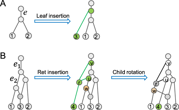
Insertion and child rotations for tree-child networks. a Leaf 3 is attached to a tree edge. b The reticulation insertion is applied to attach a new reticulate node r onto two tree edges. The child rotation swaps the tree node w (yellow) and Leaf 4. Here, green nodes and edges are added nodes
Reticulation insertion For a pair of tree edges e1=(u1,v1) and e2=(u2,v2) of N, which are not necessarily distinct, insert a new node w1 to subdivide e1 and a new node w2 to subdivide e2, attach a new reticulate node r as the common child of w1 and w2 and make Leaf (n+1) to be the child of r. In this case, we say that rstraddles e1 and e2. We use Ret-Insert(N,e1,e2,n+1) to denote the resulting network. We simply write Ret-Insert(N,e,n+1) if e1=e2=e.
Child rotation Let r be a reticulate node with parents \(u \in {\mathcal {T}}(N)\) and v. If u is not an ancestor of v, exchange the unique child of r and the other child of u. The resulting network is denoted by C-Rotate(N,u,r).

Note that a child rotation is a special case of the rNNI rearrangement introduced by Gambette et al. in [12]. Let \({\mathcal {T}CN}_{k}(n)\) denote the set of TCNs with k reticulations on [1,n].
Proposition 1
Let \(M\in {\mathcal {T}CN}_{k}(n)\) and let e1 and e2 be two tree edges of M. Then,
Proof
The second statement is a special case of the first. Let e1=(u,v) and e2=(x,y). Since e1 and e2 are tree edges, both v and y are tree nodes or leaves. Let r be the added reticulate node. Then the parents of r have v and y as their child, respectively, the nodes u and x have the parents of r as their tree node child; Leaf n+1 is the tree child r. Additionally, all the other nodes have the same children as in M. Therefore, Ret-Insert(M,e1,e2,n+1) is a TCN. □
Proposition 2
Let \(M\in {\mathcal {T}CN}_{k+1}(n+1)\). Assume that \(r\in {\mathcal {R}}(M)\) and its parents are u and v such that u is not an ancestor of v in M. Then,
Proof
Let M′=C-Rotate(M,u,r). Since u is a parent of r and M is tree-child, u is a tree node. Let w be the other child of u and let z be the unique child of r. Since M is tree-child, z and w are tree nodes (see Fig. 2). The tree node z becomes the child of u Therefore, every node also has a child that is a tree node or a leaf in M′. □
By definition, w becomes a child of r and z becomes a tree node child of u in M′. If M′ contains a directed cycle C, C must contain v and w, implying that u is an ancestor of v in M, a contradiction. Therefore, M′ is acyclic and \(M' \in {\mathcal {T}CN}_{k+1}(n+1)\).
Proposition 3
Let \(N\in {\mathcal {T}CN}_{k+1}(n+1)\).
(i) If Leaf (n+1) is the child of a reticulate node r, N can then be obtained from an \(M\in {\mathcal {T}CN}_{k}(n)\) via a reticulation insertion.
(ii) If Leaf (n+1) is the child of a tree node t and the sibling of n+1 is also a tree node, N can then obtained from an \(M\in {\mathcal {T}CN}_{k+1}(n)\) via a leaf insertion.
(iii) If Leaf (n+1) is a child of a tree node t and the sibling of n+1 is a reticulate node, N can then be obtained from an \(M\in {\mathcal {T}CN}_{k+1}(n+1)\) via a child rotation.
Proof
(i) Let r have parents u1 and u2 in N. Since N is a TCN, u1 and u2 are tree nodes and so are their children other than r. Let wi and vi be the parent and the child of ui such that vi≠r, respectively, for each i=1,2. Since r is a reticulate node, v1 and v2 are tree nodes. Without loss of generality, we assume that u2 is not the parent of u1. There are two cases for consideration.
If u1 is the parent of u2, then u1=w2 and u2=v1 (Fig. 3a). Removing Leaf (n+1),u1 and u2 (together with incident edges) and adding an edge e=(w1,v2) produce a TCN M with k reticulations such that N=Ret-Insert(M,e,n+1).

An illustration of the proof of Proposition 3. a The reticulate node parent r of n+1 has two adjacent parents. b The reticulate node parent r of n+1 has two non-adjacent parents. c The parent and sibling of n+1 are both a tree node. d The parent of n+1 is a tree node, whereas the sibling of n+1 is a reticulate node
If u1 is not the parent of u2, then, w1≠u2 (Fig. 3b). After removing Leaf n+1,u1 and u2 (together with incident edges) and adding two edges ei=(wi,vi) (i=1,2), we obtain a TCN M such that N=Ret-Insert(M,e1,e2,n+1).
(ii) Let u be the parent of t and let v be the sibling of Leaf n+1 (Fig. 3c). By assumption, v is a tree node. After removing t and Leaf (n+1) (together with incident edges) and adding e=(u,v), we obtain a TCN \(M\in {\mathcal {T}CN}_{k+1}(n)\) such that N=Leaf-Insert(M,(u,v),n+1).
(iii) Let y be the sibling of n+1 that is a reticulate node (Fig. 3d). Let z be the child of y and let M=C-Rotate(N,t,y). Since z is below y and y is below t in N, neither attaching the tree node z below t nor attaching Leaf (n+1) below y generates a directed cycle in M. Hence, \(M\in {\mathcal {T}CN}_{k+1}(n+1)\) in which Leaf (n+1) is the child of a reticulate node y such that N=C-Rotate(M,t,y). □
Proposition 4
Let \(N_{1}, N_{2} \in {\mathcal {T}CN}_{k}(n)\).
(i) Leaf-Insert(N1,e1,n+1) is identical to Leaf-Insert(N2,e2,n+1) iff N1=N2 and e1=e2.
(ii) Ret-Insert(N1,e1,e1′,n+1) is identical to Ret-Insert(N2,e2,e2′,n+1) iff N1=N2.
(iii) Assume the parent of Leaf n is a reticulate node yi in Ni for i=1,2. C-Rotate(N1,x1,y1) is identical to C-Rotate(N2,x2,y2) iff N1=N2.
Proof
(i) Let \(N_{i} \in {\mathcal {T}CN}_{k}(n)\) and \(e_{i}\in {\mathcal {V}}(N_{i}), i=1, 2\). Let M1=Leaf-Insert(N1,e1,n+1) and M2=Leaf-Insert(N2,e2,n+1) such that M1=M2. Then, there exists a node mapping ϕ from M1 to M2 such that (i) it maps a leaf in M1 to the same leaf and (ii) \((\phi (u), \phi (v))\in {\mathcal {E}}(M_{2})\) if and only if \((u, v)\in {\mathcal {E}}(M_{1})\). Since n+1 is inserted as a leaf, ϕ maps the parent p1 of (n+1) in M1 to the parent p2 of n+1 in M2, implying that ϕ induces an isomorphic mapping from N1 to N2. This proves the necessity condition. The sufficient condition is straightforward.
(ii) and (iii) Both statement can be proved similarly. The proposition is proved. □
Figure 4 show how to generate the left TCN given in Fig. 1.

Illustration how to generate the left TCN in Figure 1 from a tree on 2 taxa
Results
Main theorems
Taken together, Propositions 1–4 imply the following theorem.
Theorem 1
Each TCN of \({\mathcal {T}CN}_{k+1}(n+1)\) can be obtained from either (i) a unique TCN of \({\mathcal {T}CN}_{k+1}(n)\) by attaching Leaf n+1 to a tree edge or (ii) a unique TCN \(N\in {\mathcal {T}CN}_{k}(n)\) by applying one of the following operations:
Insertion of a reticulate node r with the child Leaf (n+1) into a tree edge or straddling two tree edges;
Insert r into a tree edge (u,v), as described in (a), and then conduct the child rotation to switch the child of r and the tree node child of v.
Insert r straddling two tree edges e′=(u′,v′) and e′′=(u′′,v′′), as described in (a), and then conduct the child rotation to switch the child of r and the tree node child of v′′ (resp. v′) if u′′ (resp. u′) is not an ancestor of u′ (resp. u′′).
If we restrict the operations on normal networks, we obtain all the normal networks in \({\mathcal {T}CN}_{k+1}(n+1)\). However, inserting a reticulate node and then applying the child rotation may lead to a scenario that a reticulation no longer satisfy the normal condition (Fig. 5). Hence, the child-rotation operation should be taken after some verification when all normal networks are enumerated.

Illustration the undesired condition in Theorem 2 that prevents from applying s a child rotation. Here, the reticulate node r and its child Leaf 4 are first inserted into the tree edges entering v1 and v2(i.e. 2) in a normal network (top), generating a normal network (middle). But, child rotation to left leads to a tree-child network that is no longer normal (bottom), in which y does not satisfy the normal condition
Theorem 2
Each normal network of \({\mathcal {T}CN}_{k+1}(n+1)\) can be obtained from either (i) a unique normal network in \({\mathcal {T}CN}_{k+1}(n)\) by attaching Leaf n+1 to a tree edge or (ii) a unique normal network \(N\in {\mathcal {T}CN}_{k}(n)\) by applying one of the following operations for each pair of incomparable edges e1=(u1,v1) and e2=(u2,v2) in N:
Insert a reticulate node r with the child (n+1) straddling e1 and e2. Let pi be the tree node inserted into ei for i=1,2.
Insert r as described in (a) and then conduct the child rotation to make v1 to be the child of r and n+1 the child of p1, respectively, unless a reticulate edge (x,y) exists in N (Fig. 5) such that:
y is below v1;
x is not an ancestor of v1;
x is an ancestor of v2.
Insert r as described in (a) and then conduct the child rotation to make v2 to be the child of r and n+1 the child of p2, respectively, unless a reticulate edge (x,y) exists in N such that:
y is below v2;
x is not an ancestor of v2;
x is an ancestor of v1.
Proof
The statement for normal networks is based on the fact that if N is obtained from N′ vis one of the three operations given in Theorem 1, that the normality of N implies the normality of N′.
The conditions in (b) and (c) are used to exclude the child rotations that make the normal condition invalid for some existing reticulate nodes in the generated TCN. □
Counting formulas
Let N be a TCN. For a pair of edges (u1,v1) and (u2,v2) of N, they are incomparable if neither of v1 and v2 is an ancestor of the other. Let u(N) be the number of unordered pairs of incomparable edges in N and let:
Define an,k to be \(|{\mathcal {T}CN}_{k}(n)|, 0\leq k< n\) and bn,k to be the number of normal networks in TCNk(n),0≤k<n.
Theorem 3
(i) The an,k can be calculated through the following recurrence formula:
where a2,0=1 and un−1,k−1 is defined in Eq. (1).
(ii) The bn,1 can be calculated through the following recurrence formula:
where un−1,0 is the total number of unordered pairs of incomparable edges in all the phylogenetic trees on n−1 taxa.
Proof
(i) The unique tree on two taxa is a TCN and thus a2,0=1.
Each TCN of \({\mathcal {T}CN}_{k}(n-1)\) has 2n+k−3 tree edges and Leaf n can be attached to each of these edges. The first term of the right hand side of Eq. (2) counts the TCNs obtained by applying the leaf insertion in Theorem 1.
Consider \(N\in {\mathcal {T}CN}_{k-1}(n-1)\). N has n−1 leaves, n+k−3 tree nodes, and thus 2n+k−4 tree edges. The reticulation insertion can be used on a single edge or a pair of edges in N. Thus, we can insert a reticulate node r with the child Leaf n in \(2n+k-4 +{2n+k-4 \choose 2}=(2n+k-3)(2n+k-4)/2\) possible ways. After the insertion of r in a tree edge (u,v), we can apply a child rotation to exchange Leaf n with v, as u is not an ancestor of v after r was inserted. Similarly, after r is connected to a pair of edges e1 and e2, we can apply a child rotation once if one edge is below the other and in two possible ways if neither is an ancestor of the other.
In summary, for each unordered pair of tree edges (e1,e2), we can generate three different tree child networks with k reticulations on [1,n] if they are incomparable and two otherwise. Thus, we have the second and third terms of the formula.
(ii) The fact that bn,n−1=0 was first proved by Bickner [25]. □
In the case that n>2 and k≤n−2, Eq. (3) for bn,1 follows from the following two facts:
Only two incomparable edges in normal networks in \({\mathcal {T}CN}_{k-1}(n-1)\) can be used to generate normal networks in \({\mathcal {T}CN}_{k}(n)\);
For each unordered pair of incomparable edges in a tree on [1,n−1], three normal networks can be obtained by applying insertion of reticulate node and two child rotations.
Unfortunately, we do not know how to obtain a simple formula for bn,k in general. By Theorem 3, one still can compute the number of normal networks with k reticulate nodes on [1,n],bn,k, by enumeration. For each 1≤k≤n−2 and 3≤n≤7,bn,k is listed in Table 1.
It is challenging to obtain a simple formula for counting un,k for arbitrary k. But we can find a closed formula for un,0 and thus obtain a recurrence formula for an,1 and bn,1.
Lemma 1
For any n≥2, the total number of unordered pairs of incomparable edges in all the phylogenetic trees on n taxa is:
Proof
Let T be a phylogenetic tree on [1,n−1] and let O(T) denote the set of ordered pairs of comparable edges in T, where that (x,y)∈O(T) means the edge x is above the edge y. Then, it is not hard to verify:
□
Assume T′ is obtained from T by attaching Leaf n in an edge e=(u,v). In T′, the parent w of Leaf n is the tree node inserted in e, implying that e is subdivided into two edges of T′:
and
Thus,
Hence,
Since T has 2n−3 edges,
where \(\mathcal {LI}(T, n)\) denotes the set of 2n−3 phylogenetic trees that are obtained by a Leaf-Insertion on T.
Let cn be the total number of unordered pairs of comparable edges in all the phylogenetic trees on n taxa. Clearly, c2=2. Since there are \(\frac {(2n-4)!}{2^{n-2}(n-2)!}\) phylogenetic trees with n−1 leaves, which each have 2n−3 edges, Eq. (5) implies:
or, equivalently,
Therefore,
where \(\frac {(2k)!}{(k+1)!k!}\) is the k-th Catalan number Ck that is equal to the integral appearing above ([31]). Since there are \(\frac {(2n-2)!}{2^{n-1}(n-1)!}\) phylogenetic trees on [1,n] each having (2n−1) edges,
Theorem 4
For any n≥3, the numbers of TCNs and normal networks with exactly one reticulate node on n taxa are:
and
respectively.
Proof
Since \(a_{n-1, 0}=\frac {(2n-4)!}{2^{n-2}(n-2)!}\), by Theorem 3,
or, equivalently,
Therefore, since a2,1=2,
By induction, we can show that \(\sum ^{n}_{k=0}{2k\choose k}4^{-k}=\frac {(2n+1)!}{2^{2n}(n!)^{2}}\) and \(\sum ^{n}_{k=0}{2k\choose k}k4^{-k}=\frac {(2n+1)!}{3\cdot 2^{2n}n!(n-1)!}\). Continuing the above calculation, we obtain:
□
This proves Eq. (6).
Similarly, by Theorem 3 and Lemma 1, we have:
or, equivalently,
Since b2,1=0,
This proves Eq. (7).
Remark 1
Every RPN with exactly one reticulate node is a TCN. Therefore, an,1 is actually the number of RPNs with one reticulate node.
Conclusions
It is well-known that all phylogenetic trees on n taxa can be generated by the insertion of the n-th taxa in each edge of all the phylogenetic trees on the first n−1 taxa. The main result of this work is a generalization of this fact into TCNs. This leads to a simple procedure for enumerating both normal networks and TCNs, the C-code for which is available upon request. It is fast enough to count all the normal networks on eight taxa. Recently, Cardona et al. introduced a novel operation to enumerate TCNs. Their program was successfully used to compute the exact number of tree-child networks on six taxa. Although our program is faster than theirs, it still cannot be used to count TCNs on eight taxa on a PC.
Another contribution of this work is Eq. (6) and (7) for counting RPNs with exactly one reticulate node. Semple and Steel [30] presented formulas for counting unrooted networks with one reticulate node. Since an unrooted networks can be oriented into a different number of RPNs, it is note clear how to use their results to derive a formula for the count of RPNs. Bouvel et al. [26] presented a formula for counting RPNs with one reticulate node. Our formula is much simpler than the formula given in [26].
Lastly, the following problem is open:
Is there a simple formula like Eq. (6) for the count of TCNs with k reticulate nodes on n taxa for each k>1?
Availability of data and materials
Data sharing is not applicable to this article as no datasets were generated or analysed during the current study.
Abbreviations
- NNI:
-
Nearest neighbor interchange
- RPN:
-
Rooted phylogenetic network
- TCN:
-
Tree-child network
References
Doolittle WF. Phylogenetic classification and the universal tree. Science. 1999; 284(5423):2124–8.
Gusfield D. ReCombinatorics: the Algorithmics of Ancestral Recombination Graphs and Explicit Phylogenetic Networks. Cambridge, USA: MIT Press; 2014.
Jain R, Rivera MC, Lake JA. Horizontal gene transfer among genomes: the complexity hypothesis. Proc Natl Acad Sci. 1999; 96(7):3801–6.
Huson DH, Rupp R, Scornavacca C. Phylogenetic Networks: Concepts, Algorithms and Applications. Cambridge, UK: Cambridge University Press; 2010.
Steel M. Phylogeny: Discrete and Random Processes in Evolution. Philadelphia, USA: SIAM; 2016.
Chor B, Tuller T. Finding a maximum likelihood tree is hard. J ACM (JACM). 2006; 53(5):722–44.
Foulds LR, Graham RL. The steiner problem in phylogeny is np-complete. Adv Appl Math. 1982; 3(1):43–9.
Felsenstein J. Inferring Phylogenies, vol. 2. Sunderland: Sinauer Associates; 2004.
Yu Y, Dong J, Liu KJ, Nakhleh L. Maximum likelihood inference of reticulate evolutionary histories. Proc Natl Acad Sci. 2014; 111(46):16448–53.
Bordewich M, Linz S, Semple C. Lost in space? Generalising subtree prune and regraft to spaces of phylogenetic networks. J Theor Biol. 2017; 423:1–12.
Francis A, Huber KT, Moulton V, Wu T. Bounds for phylogenetic network space metrics. J Math Biol. 2018; 76(5):1229–48.
Gambette P, Van Iersel L, Jones M, Lafond M, Pardi F, Scornavacca C. Rearrangement moves on rooted phylogenetic networks. PLoS Comput Biol. 2017; 13(8):1005611.
Huber KT, Linz S, Moulton V, Wu T. Spaces of phylogenetic networks from generalized nearest-neighbor interchange operations. J Math Biol. 2016; 72(3):699–725.
Huber KT, Moulton V, Wu T. Transforming phylogenetic networks: Moving beyond tree space. J Theor Biol. 2016; 404:30–9.
Janssen R, Jones M, Erdős PL, Van Iersel L, Scornavacca C. Exploring the tiers of rooted phylogenetic network space using tail moves. Bull Math Biol. 2018; 80(8):2177–208.
Klawitter J, Linz S. On the subnet prune and regraft distance. Electron J Combin. 2019; 26:2–3.
Gusfield D, Eddhu S, Langley C. The fine structure of galls in phylogenetic networks. INFORMS J Comput. 2004; 16(4):459–69.
Wang L, Zhang K, Zhang L. Perfect phylogenetic networks with recombination. J Comput Biol. 2001; 8(1):69–78.
Cardona G, Rossello F, Valiente G. IEEE/ACM Trans Comput Biol Bioinforma (TCBB). 2009; 6(4):552–569.
Willson SJ. Unique determination of some homoplasies at hybridization events. Bull Math Biol. 2007; 69(5):1709–25.
Francis AR, Steel M. Which phylogenetic networks are merely trees with additional arcs?Syst Biol. 2015; 64(5):768–77.
Zhang L. On tree-based phylogenetic networks. J Comput Biol. 2016; 23(7):553–65.
Zhang L. Clusters, trees, and phylogenetic network classes. In: Bioinformatics and Phylogenetics. New York: Springer: 2019. p. 277–315.
Gunawan AD, Yan H, Zhang L. Compression of phylogenetic networks and algorithm for the tree containment problem. J Comput Biol. 2019; 26(3):285–94.
Bickner DR. On normal networks. PhD thesis, Iowa State University, Department of Mathematics. 2012.
Bouvel M, Gambette P, Mansouri M. Counting level-k phylogenetic networks. arXiv preprint arXiv:1909.10460. 2019.
Cardona G, Pons JC, Scornavacca C. Generation of Binary Tree-Child phylogenetic networks. PLoS Computat Biol. 2019; 15(9):e1007347.
Fuchs M, Gittenberger B, Mansouri M. Counting phylogenetic networks with few reticulation vertices: tree-child and normal networks. Australas J Comb. 2019; 73(2):385–423.
McDiarmid C, Semple C, Welsh D. Counting phylogenetic networks. Ann Comb. 2015; 19(1):205–24.
Semple C, Steel M. IEEE/ACM Trans Comput Biol Bioinforma (TCBB). 2006; 3(1):84.
Stanley RP. Catalan Numbers. Cambridge, UK: Cambridge University Press; 2015.
Acknowledgements
The author thanks Mike Steel for useful discussion of counting networks and comments on the manuscript and Yurui Chen for implementing the implementation of the enumeration method given in this work. He also thanks anonymous reviewers and Jonathan Klawitter for useful feedback on the first draft of this paper.
About this supplement
This article has been published as part of BMC Bioinformatics Volume 20 Supplement 20, 2019: Proceedings of the 17th Annual Research in Computational Molecular Biology (RECOMB) Comparative Genomics Satellite Workshop: Bioinformatics. The full contents of the supplement are available online at https://bmcbioinformatics.biomedcentral.com/articles/supplements/volume-20-supplement-20.
Funding
Publication costs of this work are funded by Singapore’s Ministry of Education Academic Research Fund Tier-1 [grant R-146-000-238-114] and the National Research Fund [grant NRF2016NRF-NSFC001-026].
Author information
Authors and Affiliations
Contributions
The author conducted research and wrote the manuscript. The author read and approved the final manuscript.
Corresponding author
Ethics declarations
Ethics approval and consent to participate
This research did not involve any human subjects, human material, or human data. The ethics approval is not applicable.
Consent for publication
Not applicable.
Competing interests
The author declares that he has no competing interests.
Additional information
Publisher’s Note
Springer Nature remains neutral with regard to jurisdictional claims in published maps and institutional affiliations.
Rights and permissions
Open Access This article is distributed under the terms of the Creative Commons Attribution 4.0 International License (http://creativecommons.org/licenses/by/4.0/), which permits unrestricted use, distribution, and reproduction in any medium, provided you give appropriate credit to the original author(s) and the source, provide a link to the Creative Commons license, and indicate if changes were made. The Creative Commons Public Domain Dedication waiver (http://creativecommons.org/publicdomain/zero/1.0/) applies to the data made available in this article, unless otherwise stated.
About this article

Cite this article
Zhang, L. Generating normal networks via leaf insertion and nearest neighbor interchange. BMC Bioinformatics 20 (Suppl 20), 642 (2019). https://doi.org/10.1186/s12859-019-3209-3
Published:
DOI: https://doi.org/10.1186/s12859-019-3209-3